Deep Learning - Generating a dataset¶

This section describes how to create a dataset for supervised learning. Note that we already described how to easily load existing datasets in Datasets. However, in this chapter we will discuss in detail how to perform augmentations on these or similar datasets.

Augmentation is a common strategy in deep learning. The goal is to use an existing dataset and make it larger (possibly infinitely) by altering both the inputs and the targets in some sensible way.

Generally, we will distinguish two types of augmentations

Intensity - change the pixel intensities
Geometric - change the geometric structure of the underlying image

The reason why in our use case we split augmentations into two groups is very simple : the intensity augmentations do not change the labels, whereas the geometric ones do change our labels.

Geometric augmentations¶

The geometric augmentations are a major part of atlalign functionality. All the augmentations can be found in atlalign.zoo module. They are easily accessible to the user via the generate class method.

affine
affine_simple
control_points
edge_stretching
projective

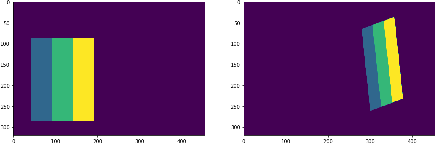
Affine simple¶

import numpy as np
import matplotlib.pyplot as plt

from atlalign.base import DisplacementField
from atlalign.data import rectangles

shape=(320, 456)

img = np.squeeze(rectangles(n_samples=1, shape=shape, height=200, width=150, random_state=31))
df = DisplacementField.generate(shape,
                                approach='affine_simple',
                                scale_x=1.9,
                                scale_y=1,
                                translation_x=-300,
                                translation_y=0,
                                rotation=0.2
                               )

img_aug = df.warp(img)

_, (ax_orig, ax_aug) = plt.subplots(1, 2, figsize=(10, 14))
ax_orig.imshow(img)
ax_aug.imshow(img_aug)

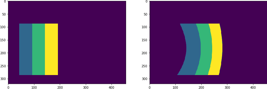
Control points¶

Control points is a generic augmentation that gives the user the possibility to specify displacement only on a selected set of control points. For the remaining pixels the displacement will be intepolation.

import matplotlib.pyplot as plt

from atlalign.base import DisplacementField
from atlalign.data import rectangles

shape = (320, 456)

img = np.squeeze(rectangles(n_samples=1, shape=shape, height=200, width=150, random_state=31))


points = np.array([[200, 150]])

values_delta_x = np.array([-100])
values_delta_y = np.array([0])

df = DisplacementField.generate(shape,
                                approach='control_points',
                                points=points,
                                values_delta_x=values_delta_x,
                                values_delta_y=values_delta_y,
                                interpolation_method='rbf')

img_aug = df.warp(img)

_, (ax_orig, ax_aug) = plt.subplots(1, 2, figsize=(10, 14))
ax_orig.imshow(img)
ax_aug.imshow(img_aug)

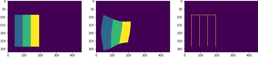
Edge stretching¶

Edge stretching using control_points in the background. However, instead of requiring the user to specify these points manually the user simply passes a mask array of edges. The algorithm then selects randomly n_perturbation_points points out of the edges and randomly displaces them. Note that the interpolation_method='rbf' and interpolator_kwargs={'function': 'linear'} gives the nicest results.

import matplotlib.pyplot as plt

from atlalign.base import DisplacementField
from atlalign.data import rectangles

from skimage.feature import canny

shape = (320, 456)

img = np.squeeze(rectangles(n_samples=1, shape=shape, height=200, width=150, random_state=31))


edge_mask = canny(img)

df = DisplacementField.generate(shape,
                                approach='edge_stretching',
                                edge_mask=edge_mask,
                                interpolation_method='rbf',
                                interpolator_kwargs={'function': 'linear'},
                                n_perturbation_points=5)

img_aug = df.warp(img)

_, (ax_orig, ax_aug, ax_edges) = plt.subplots(1, 3, figsize=(10, 14))
ax_orig.imshow(img)
ax_aug.imshow(img_aug)
ax_edges.imshow(edge_mask)

Intensity augmentations¶

Intensity augmentations do not change the label (displacement field). As opposed to the geometric ones, we fully delegate these augmentations to a 3rd party package - imgaug. For more details see the official documentation.

The user can use some preset augmentor pipeplines in atlalign.ml_utils.augmentation or create his own. See below an example of using a preset augmentor together with a small animation showing 10 random augmentations.

from atlalign.ml_utils import augmenter_1

img = np.squeeze(rectangles(n_samples=1, shape=shape, height=200, width=150, random_state=31))
aug = augmenter_1()

img_aug = aug.augment_image(img)

Make sure that imgaug pipelines do not contain any geometric transformation.

Putting things together¶

With the tools described above and the ones from Building Blocks we can significantly increase the size of our supervised learning datasets. Note that in general we want to augment the moving image with both the intensity and geometric augmentations. The reference image stays the same or only intensity augmentation is applied.

To better demonstrate the geometric augmentation logic for real data, we refer the reader to the sketch below.

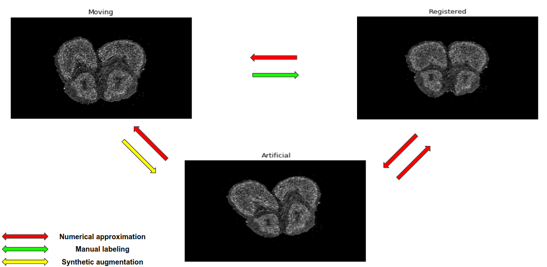
We assume that at the beginning we are given the moving image and transformation that registers this image - mov2reg (in green). Note that if only registered images are provided this is equivalent to setting mov2reg equal to an identity mapping. The actual augmentation is captured by mov2art (in yellow). Once the user specifies it (randomly generates), then atlalign can imply the art2reg. How?

Invert mov2art to obtain art2mov.
Compose art2mov and mov2reg

One clearly sees that the final transformation art2reg will be a combination of the mov2reg and art2mov. Ideally, we want to make sure that these transformations are as nice as possible - differentiable and invertible.

Note that one can inspect df.jacobian to programatically determine how smooth the transformation is. Specifically, the pixels with nonpositive jacobian represent possible artifacts. Using edge_stretching or similar it can happen occasionally that the transformations are ugly.

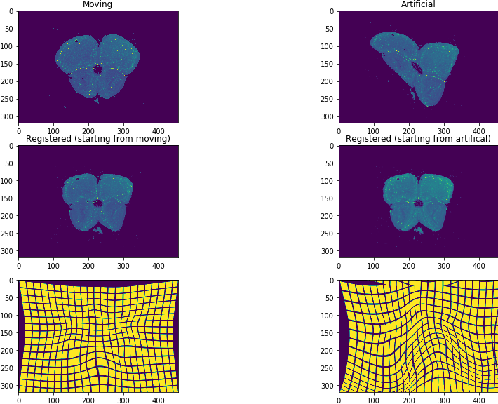
See below an end-to-end example.

Example¶

import matplotlib.pyplot as plt
import numpy as np
from skimage.feature import canny
from skimage.util import img_as_float32

from atlalign.base import DisplacementField
from atlalign.data import new_registration
from atlalign.visualization import create_grid


# helper function
def generate_mov2art(img_mov, anchor=True):
    """Generate geometric augmentation and its inverse."""
    shape = img_mov.shape
    img_mov_float = img_as_float32(img_mov)
    edge_mask = canny(img_mov_float)
    mov2art = DisplacementField.generate(shape,
                                approach='edge_stretching',
                                edge_mask=edge_mask,
                                interpolation_method='rbf',
                                interpolator_kwargs={'function': 'linear'},
                                n_perturbation_points=5)

    if anchor:
        mov2art = mov2art.anchor()

    art2mov = mov2art.pseudo_inverse()

    return mov2art, art2mov

# load datast
orig_dataset = new_registration()
i = 10

# load existing data
img_mov = orig_dataset['img'][i]
mov2reg = DisplacementField(orig_dataset['deltas_xy'][i,..., 0], orig_dataset['deltas_xy'][i,..., 1])
img_grid = create_grid(img_mov.shape)

# generate mov2art
mov2art, art2mov = generate_mov2art(img_mov)
img_art = mov2art.warp(img_mov)

# numerically approximate composition
art2reg = art2mov(mov2reg, border_mode='reflect')


# Plotting
_, ((ax_mov, ax_art),
    (ax_reg_mov, ax_reg_art),
    ( ax_reg_mov_grid, ax_reg_art_grid)) = plt.subplots(3, 2, figsize=(15, 10))


ax_mov.imshow(img_mov)
ax_mov.set_title('Moving')
ax_art.imshow(img_art)
ax_art.set_title('Artificial')

ax_reg_mov.imshow(mov2reg.warp(img_mov))
ax_reg_mov.set_title('Registered (starting from moving)')
ax_reg_art.imshow(art2reg.warp(img_art))
ax_reg_art.set_title('Registered (starting from artifical)')

ax_reg_mov_grid.imshow(mov2reg.warp(img_grid))
ax_reg_art_grid.imshow(art2reg.warp(img_grid))

Since generation of the augmentations or finding the inverse numerically might be slow we highly recommend precomputing everything in advance (before training) and storing it in a .h5 file. See the atlalign.augmentations.py module that implements a similar strategy. Note that the training logic requires the data to be stored in a .h5 file.

Source

source/deep_learning_data.rst