Building Blocks
Displacement field
The geometric transformation can be captured by a so called displacement field. It specifies pixel by pixel correspondence between the reference and moving space.
Within the package, the corresponding class is atlalign.base.DisplacementField. To instantiate it
one has two options
Provide
delta_xanddelta_y- 2D arrays of the same shape representing the displacement in the x and y directionUse the class method
generatethat provides access to wide range of predefined geometric transformations.
import numpy as np

from atlalign.base import DisplacementField

shape = (30, 35)

# Manual construction
delta_x = np.zeros(shape)
delta_y = np.zeros(shape)

df_manual = DisplacementField(delta_x, delta_y)

# Presets
df_preset = DisplacementField.generate(shape, approach='identity')

# They lead to the same result
assert df_manual == df_preset
The DisplacementField comes with multiple useful methods and attributes.
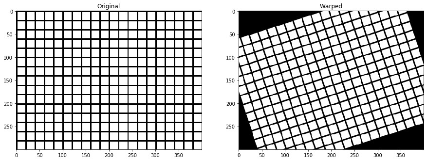
Image warping
The main operation that one can perform with a displacement field is image warping. It corresponds
to applying a given geometric transformation to an image. The corresponding method is warp.
import matplotlib.pyplot as plt
import numpy as np

from atlalign.base import DisplacementField
from atlalign.visualization import create_grid

shape = (300, 400)

df =  DisplacementField.generate(shape, approach='affine_simple', rotation=np.pi / 10)
img = create_grid(shape)
img_warped = df.warp(img)

fig, (ax_1, ax_2) = plt.subplots(1, 2, figsize=(15, 10))
ax_1.imshow(img, cmap='gray')
ax_1.set_title('Original')
ax_2.imshow(img_warped, cmap='gray')
ax_2.set_title('Warped')
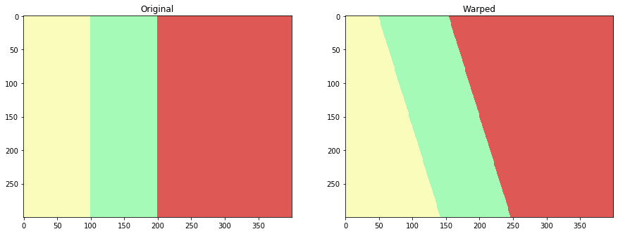
Annotation warping
Annotation warping can be used on segmentation/annotation images where each pixel represents a class rather
than an intensity. The reason why image and annotation warping are separated is that different interpolation schemes
are necessary. The corresponding method is warp_annotation.
import matplotlib.pyplot as plt
import numpy as np

from atlalign.base import DisplacementField
from atlalign.visualization import create_segmentation_image

shape = (300, 400)

annot = np.zeros(shape, dtype='int32')
annot[:, :100] = 1
annot[:, 100:200] = 321
annot[:, 200:] = 113

df = DisplacementField.generate(shape, approach='affine_simple', rotation=0.3)

warped_annot = df.warp_annotation(annot)

annot_img, colors_dict = create_segmentation_image(annot)
warped_annot_img = create_segmentation_image(warped_annot, colors_dict=colors_dict)[0]

assert set(np.unique(annot)) == set(np.unique(warped_annot))

fig, (ax_1, ax_2) = plt.subplots(1, 2, figsize=(15, 10))
ax_1.imshow(annot_img)
ax_1.set_title('Original')
ax_2.imshow(warped_annot_img)
ax_2.set_title('Warped')
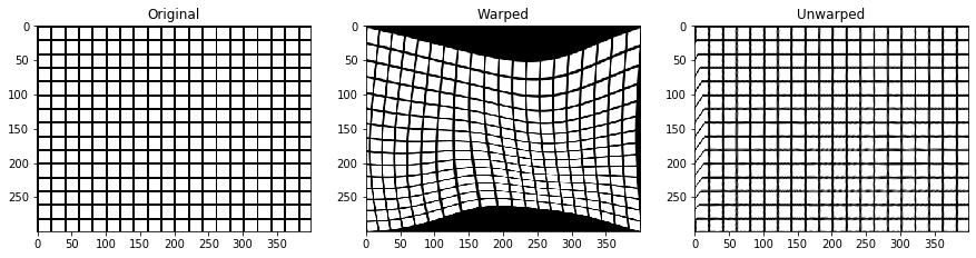
Inversion
Once given a displacement field we can find its inverse (numerically). Note that inversion is a necessary operation when
creating artificial augmentations. If we warp an image with a given displacement field, we need to also know the way
how to undo it. The corresponding method is pseudo_inverse.
import matplotlib.pyplot as plt
import numpy as np

from atlalign.base import DisplacementField
from atlalign.visualization import create_grid

shape = (300, 400)
edge_mask = np.zeros(shape, dtype=bool)
edge_mask[200:250, 100:300] = True


df =  DisplacementField.generate(shape,
                                 approach='edge_stretching',
                                 edge_mask=edge_mask,
                                 n_perturbation_points=4,
                                 radius_max=20,
                                 interpolation_method='rbf')
df_inv = df.pseudo_inverse()

img = create_grid(shape)
img_warped = df.warp(img)
img_unwarped = df_inv.warp(img_warped)

fig, (ax_1, ax_2, ax_3) = plt.subplots(1, 3, figsize=(15, 10))
ax_1.imshow(img, cmap='gray')
ax_1.set_title('Original')
ax_2.imshow(img_warped, cmap='gray')
ax_2.set_title('Warped')
ax_3.imshow(img_unwarped, cmap='gray')
ax_3.set_title('Unwarped')
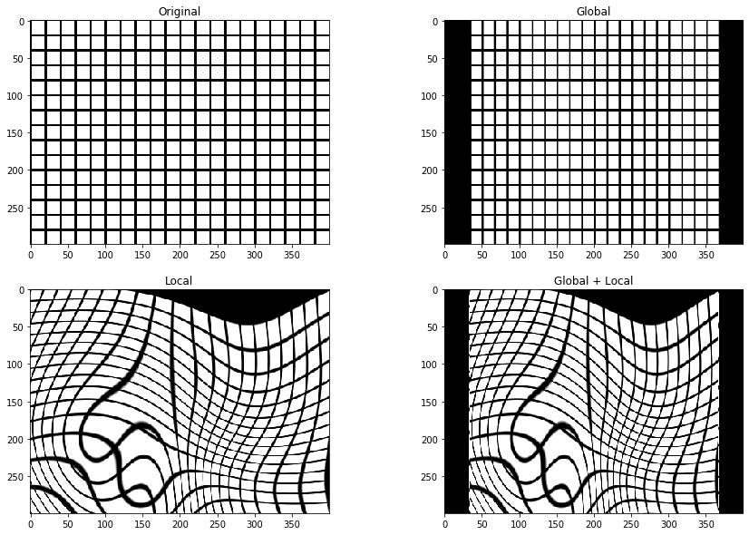
Composition
For more sophisticated augmentations it is useful combine multiple different transformations. This corresponds
to composition of displacement fields. The corresponding method is __call__.
import matplotlib.pyplot as plt
import numpy as np

from atlalign.base import DisplacementField
from atlalign.visualization import create_grid

shape = (300, 400)
edge_mask = np.zeros(shape, dtype=bool)
edge_mask[200:250, 100:300] = True


df_g = DisplacementField.generate(shape, approach='affine_simple', scale_x=1.2)

df_l = DisplacementField.generate(shape,
                                 approach='edge_stretching',
                                 edge_mask=edge_mask,
                                 n_perturbation_points=5,
                                 radius_max=50,
                                 interpolation_method='rbf')

df_gl = df_l(df_g)

img = create_grid(shape)
img_warped_g = df_g.warp(img)
img_warped_l = df_l.warp(img)
img_warped_gl = df_gl.warp(img)

fig, ((ax_1, ax_2), (ax_3, ax_4)) = plt.subplots(2, 2, figsize=(15, 10))

ax_1.imshow(img, cmap='gray')
ax_1.set_title('Original')

ax_2.imshow(img_warped_g, cmap='gray')
ax_2.set_title('Global')

ax_3.imshow(img_warped_l, cmap='gray')
ax_3.set_title('Local')

ax_4.imshow(img_warped_gl, cmap='gray')
ax_4.set_title('Global + Local')
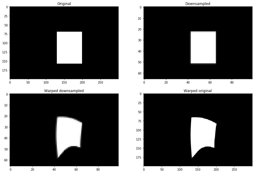
Resizing
For performance purposes it might beneficial to downsample the moving image and then perform registration. Once it is
done one can resize the displacement field and warp the original image to get higher resolution images. Note that this
trick will yield superior results of simply upsampling the registered image.
The corresponding method is resize_constant.
import matplotlib.pyplot as plt
import numpy as np
from skimage.draw import rectangle
from skimage.feature import canny
from skimage.transform import resize

from atlalign.base import DisplacementField

original_shape = (200, 300)
new_shape = (66, 99)

img_original = np.zeros(original_shape, dtype='float32')

start = (70, 130)
extent = (88, 70)

rr, cc = rectangle(start, extent=extent, shape=img_original.shape)

img_original[rr, cc] = 1
img_new = resize(img_original, new_shape)

edge_mask = canny(img_new)
df =  DisplacementField.generate(new_shape,
                                 approach='edge_stretching',
                                 edge_mask=edge_mask,
                                 n_perturbation_points=5,
                                 radius_max=5,
                                 interpolation_method='rbf')

df_resized = df.resize_constant(original_shape)

img_new_warped = df.warp(img_new)
img_original_warped = df_resized.warp(img_original)


fig, ((ax_1, ax_2), (ax_3, ax_4)) = plt.subplots(2, 2, figsize=(15, 10))

ax_1.imshow(img_original, cmap='gray')
ax_1.set_title('Original')

ax_2.imshow(img_new, cmap='gray')
ax_2.set_title('Downsampled')

ax_3.imshow(img_new_warped, cmap='gray')
ax_3.set_title('Warped downsampled')

ax_4.imshow(img_original_warped, cmap='gray')
ax_4.set_title('Warped original')
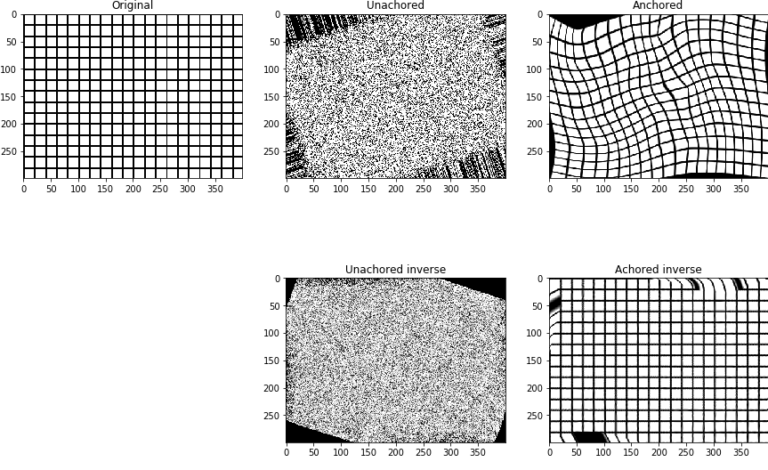
Anchoring
In general, the geometric transformations do not have to be well behaved. Two common problems are the following:
The transformation around the 4 corners of an image might not be close to an identity mapping
The transformations are not smooth enough
Both of the mentioned problems can result in difficulties when computing inverses numerically. To remove partially or
completely these undesirable features one can use the anchor method.
import matplotlib.pyplot as plt
import numpy as np

from atlalign.base import DisplacementField
from atlalign.visualization import create_grid

shape = (300, 400)

df_rotation = DisplacementField.generate(shape, approach='affine_simple', rotation=np.pi / 10)
df_ugly= DisplacementField(np.random.randint(-20, 20, size=shape),np.random.randint(-20, 20, size=shape))

df_unanchored = df_ugly(df_rotation)
df_anchored = df_unanchored.anchor(smooth=0, ds_f=50)

df_unanchored_inv = df_unanchored.pseudo_inverse()
df_anchored_inv = df_anchored.pseudo_inverse()

img = create_grid(shape)

fig, ((ax_1, ax_2, ax_3), (ax_4, ax_5, ax_6)) = plt.subplots(2, 3, figsize=(15, 10))
ax_1.imshow(img, cmap='gray')
ax_1.set_title('Original')
ax_2.imshow(df_unanchored.warp(img), cmap='gray')
ax_2.set_title('Unachored')
ax_3.imshow(df_anchored.warp(img), cmap='gray')
ax_3.set_title('Anchored')

ax_4.set_axis_off()
ax_5.imshow(df_unanchored_inv.warp(df_unanchored.warp(img)),  cmap='gray')
ax_5.set_title('Unachored inverse')
ax_6.imshow(df_anchored_inv.warp(df_anchored.warp(img)), cmap='gray')
ax_6.set_title('Achored inverse')